


0️⃣ 前言
本章思维导图:

0️⃣.1️⃣ 赛题重述
这是一道来自于天池的新手练习题目,用数据分析、机器学习等手段进行 二手车售卖价格预测 的回归问题。赛题本身的思路清晰明了,即对给定的数据集进行分析探讨,然后设计模型运用数据进行训练,测试模型,最终给出选手的预测结果。前面我们已经进行过EDA分析在这里天池_二手车价格预测_Task1-2_赛题理解与数据分析
以及天池_二手车价格预测_Task3_特征工程
0️⃣.2️⃣ 数据集概述
赛题官方给出了来自Ebay Kleinanzeigen的二手车交易记录,总数据量超过40w,包含31列变量信息,其中15列为匿名变量,即v0至v15。并从中抽取15万条作为训练集,5万条作为测试集A,5万条作为测试集B,同时对name、model、brand和regionCode等信息进行脱敏。具体的数据表如下图:
| Field | Description |
|---|---|
| SaleID | 交易ID,唯一编码 |
| name | 汽车交易名称,已脱敏 |
| regDate | 汽车注册日期,例如20160101,2016年01月01日 |
| model | 车型编码,已脱敏 |
| brand | 汽车品牌,已脱敏 |
| bodyType | 车身类型:豪华轿车:0,微型车:1,厢型车:2,大巴车:3,敞篷车:4,双门汽车:5,商务车:6,搅拌车:7 |
| fuelType | 燃油类型:汽油:0,柴油:1,液化石油气:2,天然气:3,混合动力:4,其他:5,电动:6 |
| gearbox | 变速箱:手动:0,自动:1 |
| power | 发动机功率:范围 [ 0, 600 ] |
| kilometer | 汽车已行驶公里,单位万km |
| notRepairedDamage | 汽车有尚未修复的损坏:是:0,否:1 |
| regionCode | 地区编码,已脱敏 |
| seller | 销售方:个体:0,非个体:1 |
| offerType | 报价类型:提供:0,请求:1 |
| creatDate | 汽车上线时间,即开始售卖时间 |
| price | 二手车交易价格(预测目标) |
| v系列特征 | 匿名特征,包含v0-14在内15个匿名特征 |
1️⃣ 数据处理
为了后面处理数据提高性能,所以需要对其进行内存优化。
- 导入相关的库
import pandas as pd
import numpy as np
import warnings
warnings.filterwarnings('ignore')
- 通过调整数据类型,帮助我们减少数据在内存中占用的空间
def reduce_mem_usage(df):
    """ 迭代dataframe的所有列,修改数据类型来减少内存的占用
    """
    start_mem = df.memory_usage().sum()
    print('Memory usage of dataframe is {:.2f} MB'.format(start_mem))

    for col in df.columns:
        col_type = df[col].dtype

        if col_type != object:
            c_min = df[col].min()
            c_max = df[col].max()
            if str(col_type)[:3] == 'int': # 判断可以用哪种整型就可以表示,就转换到那个整型去
                if c_min > np.iinfo(np.int8).min and c_max < np.iinfo(np.int8).max:
                    df[col] = df[col].astype(np.int8)
                elif c_min > np.iinfo(np.int16).min and c_max < np.iinfo(np.int16).max:
                    df[col] = df[col].astype(np.int16)
                elif c_min > np.iinfo(np.int32).min and c_max < np.iinfo(np.int32).max:
                    df[col] = df[col].astype(np.int32)
                elif c_min > np.iinfo(np.int64).min and c_max < np.iinfo(np.int64).max:
                    df[col] = df[col].astype(np.int64)
            else:
                if c_min > np.finfo(np.float16).min and c_max < np.finfo(np.float16).max:
                    df[col] = df[col].astype(np.float16)
                elif c_min > np.finfo(np.float32).min and c_max < np.finfo(np.float32).max:
                    df[col] = df[col].astype(np.float32)
                else:
                    df[col] = df[col].astype(np.float64)
        else:
            df[col] = df[col].astype('category')

    end_mem = df.memory_usage().sum()
    print('Memory usage after optimization is: {:.2f} MB'.format(end_mem))
    print('Decreased by {:.1f}%'.format(100 * (start_mem - end_mem) / start_mem))
    return df
sample_feature = reduce_mem_usage(pd.read_csv('../excel/data_for_tree.csv'))
Memory usage of dataframe is 35249888.00 MB
Memory usage after optimization is: 8925652.00 MB
Decreased by 74.7%
continuous_feature_names = [x for x in sample_feature.columns if x not in ['price','brand','model']]
sample_feature.head()
| SaleID | name | model | brand | bodyType | fuelType | gearbox | power | kilometer | notRepairedDamage | ... | used_time | city | brand_amount | brand_price_max | brand_price_median | brand_price_min | brand_price_sum | brand_price_std | brand_price_average | power_bin | |
|---|---|---|---|---|---|---|---|---|---|---|---|---|---|---|---|---|---|---|---|---|---|
| 0 | 1 | 2262 | 40.0 | 1 | 2.0 | 0.0 | 0.0 | 0 | 15.0 | - | ... | 4756.0 | 4.0 | 4940.0 | 9504.0 | 3000.0 | 149.0 | 17934852.0 | 2538.0 | 3630.0 | NaN |
| 1 | 5 | 137642 | 24.0 | 10 | 0.0 | 1.0 | 0.0 | 109 | 10.0 | 0.0 | ... | 2482.0 | 3.0 | 3556.0 | 9504.0 | 2490.0 | 200.0 | 10936962.0 | 2180.0 | 3074.0 | 10.0 |
| 2 | 7 | 165346 | 26.0 | 14 | 1.0 | 0.0 | 0.0 | 101 | 15.0 | 0.0 | ... | 6108.0 | 4.0 | 8784.0 | 9504.0 | 1350.0 | 13.0 | 17445064.0 | 1798.0 | 1986.0 | 10.0 |
| 3 | 10 | 18961 | 19.0 | 9 | 3.0 | 1.0 | 0.0 | 101 | 15.0 | 0.0 | ... | 3874.0 | 1.0 | 4488.0 | 9504.0 | 1250.0 | 55.0 | 7867901.0 | 1557.0 | 1753.0 | 10.0 |
| 4 | 13 | 8129 | 65.0 | 1 | 0.0 | 0.0 | 0.0 | 150 | 15.0 | 1.0 | ... | 4152.0 | 3.0 | 4940.0 | 9504.0 | 3000.0 | 149.0 | 17934852.0 | 2538.0 | 3630.0 | 14.0 |
5 rows × 39 columns
continuous_feature_names
['SaleID',
 'name',
 'bodyType',
 'fuelType',
 'gearbox',
 'power',
 'kilometer',
 'notRepairedDamage',
 'seller',
 'offerType',
 'v_0',
 'v_1',
 'v_2',
 'v_3',
 'v_4',
 'v_5',
 'v_6',
 'v_7',
 'v_8',
 'v_9',
 'v_10',
 'v_11',
 'v_12',
 'v_13',
 'v_14',
 'train',
 'used_time',
 'city',
 'brand_amount',
 'brand_price_max',
 'brand_price_median',
 'brand_price_min',
 'brand_price_sum',
 'brand_price_std',
 'brand_price_average',
 'power_bin']
2️⃣ 线性回归
2️⃣.1️⃣ 简单建模
设置训练集的自变量train_X与因变量train_y
sample_feature = sample_feature.dropna().replace('-', 0).reset_index(drop=True)
sample_feature['notRepairedDamage'] = sample_feature['notRepairedDamage'].astype(np.float32)

train = sample_feature[continuous_feature_names + ['price']]
train_X = train[continuous_feature_names]
train_y = train['price']
- 从
sklearn.linear_model库调用线性回归函数
from sklearn.linear_model import LinearRegression
训练模型,normalize设置为True则输入的样本数据将$$\frac{(X-X_)}{||X||}$$
model = LinearRegression(normalize=True)
model = model.fit(train_X, train_y)
查看训练的线性回归模型的截距(intercept)与权重(coef),其中zip先将特征与权重拼成元组,再用dict.items()将元组变成列表,lambda里面取元组的第2个元素,也就是按照权重排序。
print('intercept:'+ str(model.intercept_))

sorted(dict(zip(continuous_feature_names, model.coef_)).items(), key=lambda x:x[1], reverse=True)
intercept:-74792.9734982533


[('v_6', 1409712.605060366),
 ('v_8', 610234.5713666412),
 ('v_2', 14000.150601494915),
 ('v_10', 11566.15879987477),
 ('v_7', 4359.400479384727),
 ('v_3', 734.1594753553514),
 ('v_13', 429.31597053081543),
 ('v_14', 113.51097451363385),
 ('bodyType', 53.59225499923475),
 ('fuelType', 28.70033988480179),
 ('power', 14.063521207625223),
 ('city', 11.214497244626225),
 ('brand_price_std', 0.26064581249034796),
 ('brand_price_median', 0.2236946027016186),
 ('brand_price_min', 0.14223892840381142),
 ('brand_price_max', 0.06288317241689621),
 ('brand_amount', 0.031481415743174694),
 ('name', 2.866003063271253e-05),
 ('SaleID', 1.5357186544049832e-05),
 ('gearbox', 8.527422323822975e-07),
 ('train', -3.026798367500305e-08),
 ('offerType', -2.0873267203569412e-07),
 ('seller', -8.426140993833542e-07),
 ('brand_price_sum', -4.1644253886318015e-06),
 ('brand_price_average', -0.10601622599106471),
 ('used_time', -0.11019174518618283),
 ('power_bin', -64.74445582883024),
 ('kilometer', -122.96508938774225),
 ('v_0', -317.8572907738245),
 ('notRepairedDamage', -412.1984812088826),
 ('v_4', -1239.4804712396635),
 ('v_1', -2389.3641453624136),
 ('v_12', -12326.513672033445),
 ('v_11', -16921.982011390297),
 ('v_5', -25554.951071390704),
 ('v_9', -26077.95662717417)]
2️⃣.2️⃣ 处理长尾分布
长尾分布是尾巴很长的分布。那么尾巴很长很厚的分布有什么特殊的呢?有两方面:一方面,这种分布会使得你的采样不准,估值不准,因为尾部占了很大部分。另一方面,尾部的数据少,人们对它的了解就少,那么如果它是有害的,那么它的破坏力就非常大,因为人们对它的预防措施和经验比较少。实际上,在稳定分布家族中,除了正态分布,其他均为长尾分布。
随机找个特征,用随机下标选取一定的数观测预测值与真实值之间的差别
from matplotlib import pyplot as plt
subsample_index = np.random.randint(low=0, high=len(train_y), size=50)

plt.scatter(train_X['v_6'][subsample_index], train_y[subsample_index], color='black')
plt.scatter(train_X['v_6'][subsample_index], model.predict(train_X.loc[subsample_index]), color='red')
plt.xlabel('v_6')
plt.ylabel('price')
plt.legend(['True Price','Predicted Price'],loc='upper right')
print('真实价格与预测价格差距过大!')
plt.show()
真实价格与预测价格差距过大!


<Figure size 640x480 with 1 Axes>
绘制特征v_6的值与标签的散点图,图片发现模型的预测结果(红色点)与真实标签(黑色点)的分布差异较大,且部分预测值出现了小于0的情况,说明我们的模型存在一些问题。
下面可以通过作图我们看看数据的标签(price)的分布情况
import seaborn as sns
plt.figure(figsize=(15,5))
plt.subplot(1,2,1)
sns.distplot(train_y)
plt.subplot(1,2,2)
sns.distplot(train_y[train_y < np.quantile(train_y, 0.9)])# 去掉尾部10%的数再画一次,依然是呈现长尾分布
<matplotlib.axes._subplots.AxesSubplot at 0x210469a20f0>
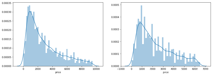
从这两个频率分布直方图来看,price呈现长尾分布,不利于我们的建模预测,原因是很多模型都假设数据误差项符合正态分布,而长尾分布的数据违背了这一假设。
在这里我们对train_y进行了$log(x+1)$变换,使标签贴近于正态分布
train_y_ln = np.log(train_y + 1)
plt.figure(figsize=(15,5))
plt.subplot(1,2,1)
sns.distplot(train_y_ln)
plt.subplot(1,2,2)
sns.distplot(train_y_ln[train_y_ln < np.quantile(train_y_ln, 0.9)])
<matplotlib.axes._subplots.AxesSubplot at 0x21046aa7588>
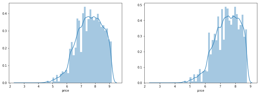
可以看出经过对数处理后,长尾分布的效果减弱了。再进行一次线性回归:
model = model.fit(train_X, train_y_ln)

print('intercept:'+ str(model.intercept_))
sorted(dict(zip(continuous_feature_names, model.coef_)).items(), key=lambda x:x[1], reverse=True)
intercept:22.237755141260187


[('v_1', 5.669305855573455),
 ('v_5', 4.244663233260515),
 ('v_12', 1.2018270333465797),
 ('v_13', 1.1021805892566767),
 ('v_10', 0.9251453991435046),
 ('v_2', 0.8276319426702504),
 ('v_9', 0.6011701859510072),
 ('v_3', 0.4096252333799574),
 ('v_0', 0.08579322268709569),
 ('power_bin', 0.013581489882378468),
 ('bodyType', 0.007405158753814581),
 ('power', 0.0003639122482301998),
 ('brand_price_median', 0.0001295023112073966),
 ('brand_price_max', 5.681812615719255e-05),
 ('brand_price_std', 4.2637652140444604e-05),
 ('brand_price_sum', 2.215129563552113e-09),
 ('gearbox', 7.094911325111752e-10),
 ('seller', 2.715054847612919e-10),
 ('offerType', 1.0291500984749291e-10),
 ('train', -2.2282620193436742e-11),
 ('SaleID', -3.7349069125800904e-09),
 ('name', -6.100613320903764e-08),
 ('brand_amount', -1.63362003323235e-07),
 ('used_time', -2.9274637535648837e-05),
 ('brand_price_min', -2.97497751376125e-05),
 ('brand_price_average', -0.0001181124521449396),
 ('fuelType', -0.0018817210167693563),
 ('city', -0.003633315365347111),
 ('v_14', -0.02594698320698149),
 ('kilometer', -0.03327227857575015),
 ('notRepairedDamage', -0.27571086049472),
 ('v_4', -0.6724689959780609),
 ('v_7', -1.178076244244115),
 ('v_11', -1.3234586342526309),
 ('v_8', -83.08615946716786),
 ('v_6', -315.0380673447196)]
再一次画出预测与真实值的散点对比图:
plt.scatter(train_X['v_6'][subsample_index], train_y[subsample_index], color='black')
plt.scatter(train_X['v_6'][subsample_index], np.exp(model.predict(train_X.loc[subsample_index])), color='blue')
plt.xlabel('v_6')
plt.ylabel('price')
plt.legend(['True Price','Predicted Price'],loc='upper right')
plt.show()
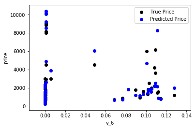
效果稍微好了一点,但毕竟是线性回归,拟合得还是不够好。
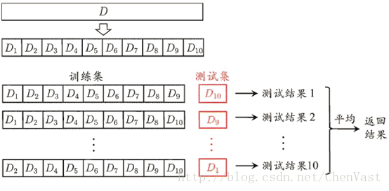
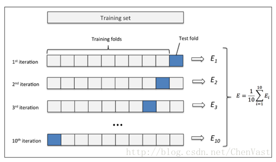
3️⃣ 五折交叉验证¶(cross_val_score)
在使用训练集对参数进行训练的时候,经常会发现人们通常会将一整个训练集分为三个部分(比如mnist手写训练集)。一般分为:训练集(train_set),评估集(valid_set),测试集(test_set)这三个部分。这其实是为了保证训练效果而特意设置的。其中测试集很好理解,其实就是完全不参与训练的数据,仅仅用来观测测试效果的数据。而训练集和评估集则牵涉到下面的知识了。
因为在实际的训练中,训练的结果对于训练集的拟合程度通常还是挺好的(初始条件敏感),但是对于训练集之外的数据的拟合程度通常就不那么令人满意了。因此我们通常并不会把所有的数据集都拿来训练,而是分出一部分来(这一部分不参加训练)对训练集生成的参数进行测试,相对客观的判断这些参数对训练集之外的数据的符合程度。这种思想就称为交叉验证(Cross Validation)。
直观的类比就是训练集是上课,评估集是平时的作业,而测试集是最后的期末考试。😏
Cross Validation:简言之,就是进行多次train_test_split划分;每次划分时,在不同的数据集上进行训练、测试评估,从而得出一个评价结果;如果是5折交叉验证,意思就是在原始数据集上,进行5次划分,每次划分进行一次训练、评估,最后得到5次划分后的评估结果,一般在这几次评估结果上取平均得到最后的评分。k-fold cross-validation ,其中,k一般取5或10。
一般情况将K折交叉验证用于模型调优,找到使得模型泛化性能最优的超参值。找到后,在全部训练集上重新训练模型,并使用独立测试集对模型性能做出最终评价。K折交叉验证使用了无重复抽样技术的好处:每次迭代过程中每个样本点只有一次被划入训练集或测试集的机会。
更多参考资料:几种交叉验证(cross validation)方式的比较
、k折交叉验证
- 下面调用
sklearn.model_selection的cross_val_score进行交叉验证
from sklearn.model_selection import cross_val_score
from sklearn.metrics import mean_absolute_error,  make_scorer
3️⃣.1️⃣ cross_val_score相应函数的应用
def log_transfer(func):
    def wrapper(y, yhat):
        result = func(np.log(y), np.nan_to_num(np.log(yhat)))
        return result
    return wrapper
-
上面的
log_transfer是提供装饰器功能,是为了将下面的cross_val_score的make_scorer的mean_absolute_error(它的公式在下面)的输入参数做对数处理,其中np.nan_to_num顺便将nan转变为0。
$$
MAE=\frac{\sum\limits_^\left|y_-\hat_\right|}
$$ -
cross_val_score是sklearn用于交叉验证评估分数的函数,前面几个参数很明朗,后面几个参数需要解释一下。verbose:详细程度,也就是是否输出进度信息cv:交叉验证生成器或可迭代的次数scoring:调用用来评价的方法,是score越大约好,还是loss越小越好,默认是loss。这里调用了mean_absolute_error,只是在调用之前先进行了log_transfer的装饰,然后调用的y和yhat,会自动将cross_val_score得到的X和y代入。make_scorer:构建一个完整的定制scorer函数,可选参数greater_is_better,默认为False,也就是loss越小越好
-
下面是对未进行对数处理的原特征数据进行五折交叉验证
scores = cross_val_score(model, X=train_X, y=train_y, verbose=1, cv = 5, scoring=make_scorer(log_transfer(mean_absolute_error)))
[Parallel(n_jobs=1)]: Using backend SequentialBackend with 1 concurrent workers.
[Parallel(n_jobs=1)]: Done   5 out of   5 | elapsed:    0.2s finished
print('AVG:', np.mean(scores))
AVG: 0.7533845471636889
scores = pd.DataFrame(scores.reshape(1,-1)) # 转化成一行,(-1,1)为一列
scores.columns = ['cv' + str(x) for x in range(1, 6)]
scores.index = ['MAE']
scores
| cv1 | cv2 | cv3 | cv4 | cv5 | |
|---|---|---|---|---|---|
| MAE | 0.727867 | 0.759451 | 0.781238 | 0.750681 | 0.747686 |
使用线性回归模型,对进行过对数处理的原特征数据进行五折交叉验证
scores = cross_val_score(model, X=train_X, y=train_y_ln, verbose=1, cv = 5, scoring=make_scorer(mean_absolute_error))
[Parallel(n_jobs=1)]: Using backend SequentialBackend with 1 concurrent workers.
[Parallel(n_jobs=1)]: Done   5 out of   5 | elapsed:    0.1s finished
print('AVG:', np.mean(scores))
AVG: 0.2124134663602803
scores = pd.DataFrame(scores.reshape(1,-1))
scores.columns = ['cv' + str(x) for x in range(1, 6)]
scores.index = ['MAE']
scores
| cv1 | cv2 | cv3 | cv4 | cv5 | |
|---|---|---|---|---|---|
| MAE | 0.208238 | 0.212408 | 0.215933 | 0.210742 | 0.214747 |
可以看出进行对数处理后,五折交叉验证的loss显著降低。
3️⃣.2️⃣ 考虑真实世界限制
例如:通过2018年的二手车价格预测2017年的二手车价格,这显然是不合理的,因此我们还可以采用时间顺序对数据集进行分隔。在本例中,我们选用靠前时间的4/5样本当作训练集,靠后时间的1/5当作验证集,最终结果与五折交叉验证差距不大。
import datetime
sample_feature = sample_feature.reset_index(drop=True)
split_point = len(sample_feature) // 5 * 4

train = sample_feature.loc[:split_point].dropna()
val = sample_feature.loc[split_point:].dropna()

train_X = train[continuous_feature_names]
train_y_ln = np.log(train['price'])
val_X = val[continuous_feature_names]
val_y_ln = np.log(val['price'])
model = model.fit(train_X, train_y_ln)
mean_absolute_error(val_y_ln, model.predict(val_X))
0.21498301182417004
3️⃣.3️⃣ 绘制学习率曲线与验证曲线
学习曲线是一种用来判断训练模型的一种方法,它会自动把训练样本的数量按照预定的规则逐渐增加,然后画出不同训练样本数量时的模型准确度。
我们可以把$J_(\theta)$和$J_(\theta)$作为纵坐标,画出与训练集数据集$m$的大小关系,这就是学习曲线。通过学习曲线,可以直观地观察到模型的准确性和训练数据大小的关系。 我们可以比较直观的了解到我们的模型处于一个什么样的状态,如:过拟合(overfitting)或欠拟合(underfitting)
如果数据集的大小为$m$,则通过下面的流程即可画出学习曲线:
-
1.把数据集分成训练数据集和交叉验证集(可以看作测试集);
-
2.取训练数据集的20%作为训练样本,训练出模型参数;
-
3.使用交叉验证集来计算训练出来的模型的准确性;
-
4.以训练集的score和交叉验证集score为纵坐标(这里的score取决于你使用的
make_score方法,例如MAE),训练集的个数作为横坐标,在坐标轴上画出上述步骤计算出来的模型准确性; -
5.训练数据集增加10%,调到步骤2,继续执行,知道训练数据集大小为100%。
learning_curve():这个函数主要是用来判断(可视化)模型是否过拟合的。下面是一些参数的解释:
X:是一个m*n的矩阵,m:数据数量,n:特征数量;y:是一个m*1的矩阵,m:数据数量,相对于X的目标进行分类或回归;groups:将数据集拆分为训练/测试集时使用的样本的标签分组。[可选];train_sizes:指定训练样品数量的变化规则。比如:np.linspace(0.1, 1.0, 5)表示把训练样品数量从0.1-1分成5等分,生成[0.1, 0.325,0.55,0.75,1]的序列,从序列中取出训练样品数量百分比,逐个计算在当前训练样本数量情况下训练出来的模型准确性。cv:None,要使用默认的三折交叉验证(v0.22版本中将改为五折);n_jobs:要并行运行的作业数。None表示1。 -1表示使用所有处理器;pre_dispatch:并行执行的预调度作业数(默认为全部)。该选项可以减少分配的内存。该字符串可以是“ 2 * n_jobs”之类的表达式;shuffle:bool,是否在基于train_sizes为前缀之前对训练数据进行洗牌;
from sklearn.model_selection import learning_curve, validation_curve
plt.fill_between()用来填充两条线间区域,其他好像没什么好解释的了。
def plot_learning_curve(estimator, title, X, y, ylim=None, cv=None,n_jobs=1, train_size=np.linspace(.1, 1.0, 5 )):
    plt.figure()
    plt.title(title)
    if ylim is not None:
        plt.ylim(*ylim)
    plt.xlabel('Training example')
    plt.ylabel('score')
    train_sizes, train_scores, test_scores = learning_curve(estimator, X, y, cv=cv, n_jobs=n_jobs, train_sizes=train_size, scoring = make_scorer(mean_absolute_error))
    train_scores_mean = np.mean(train_scores, axis=1)
    train_scores_std = np.std(train_scores, axis=1)
    test_scores_mean = np.mean(test_scores, axis=1)
    test_scores_std = np.std(test_scores, axis=1)
    plt.grid()#区域
    plt.fill_between(train_sizes, train_scores_mean - train_scores_std,
                     train_scores_mean + train_scores_std, alpha=0.1,
                     color="r")
    plt.fill_between(train_sizes, test_scores_mean - test_scores_std,
                     test_scores_mean + test_scores_std, alpha=0.1,
                     color="g")
    plt.plot(train_sizes, train_scores_mean, 'o-', color='r',
             label="Training score")
    plt.plot(train_sizes, test_scores_mean,'o-',color="g",
             label="Cross-validation score")
    plt.legend(loc="best")
    return plt
plot_learning_curve(LinearRegression(), 'Liner_model', train_X[:], train_y_ln[:], ylim=(0.0, 0.5), cv=5, n_jobs=-1)
<module 'matplotlib.pyplot' from 'D:\\Software\\Anaconda\\lib\\site-packages\\matplotlib\\pyplot.py'>
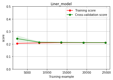
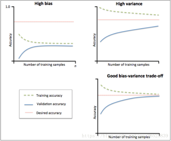
训练误差与验证误差逐渐一致,准确率也挺高(这里的score是MAE,所以是loss趋近于0.2,准确率趋近于0.8),但是训练误差几乎没变过,所以属于过拟合。这里给出一下高偏差欠拟合(bias)以及高方差过拟合(variance)的模样:
更形象一点:
Data:
Normal fitting:
overfitting:
serious overfitting:
4️⃣ 多种模型对比
train = sample_feature[continuous_feature_names + ['price']].dropna()

train_X = train[continuous_feature_names]
train_y = train['price']
train_y_ln = np.log(train_y + 1)
4️⃣.1️⃣ 线性模型 & 嵌入式特征选择
有一些前叙知识需要补全。其中关于正则化的知识:
- 分别为L1正则化与L2正则化;
- L1正则化的模型建叫做Lasso回归,使用L2正则化的模型叫做Ridge回归(岭回归);
- L1正则化是指权值向量w中各个元素的绝对值之和,通常表示为$\left | w \right | _{1} $;
- L2正则化是指权值向量w中各个元素的平方和然后再求平方根(可以看到Ridge回归的L2正则化项有平方符号),通常表示为$\left | w \right | _{2} $
- L1正则化可以产生稀疏权值矩阵,即产生一个稀疏模型,可以用于特征选择;
- L2正则化可以防止模型过拟合(overfitting),一定程度上,L1也可以防止过拟合;
更多其他知识可以看这篇文章:机器学习中正则化项L1和L2的直观理解
在过滤式和包裹式特征选择方法中,特征选择过程与学习器训练过程有明显的分别。而嵌入式特征选择在学习器训练过程中自动地进行特征选择。嵌入式选择最常用的是L1正则化与L2正则化。在对线性回归模型加入两种正则化方法后,他们分别变成了岭回归与Lasso回归。
4️⃣.1️⃣.1️⃣ LinearRegression,Ridge,Lasso方法的运行
from sklearn.linear_model import LinearRegression
from sklearn.linear_model import Ridge
from sklearn.linear_model import Lasso
models = [LinearRegression(),
          Ridge(),
          Lasso()]
result = dict()
for model in models:
    model_name = str(model).split('(')[0]
    scores = cross_val_score(model, X=train_X, y=train_y_ln, verbose=0, cv = 5, scoring=make_scorer(mean_absolute_error))
    result[model_name] = scores
    print(model_name + ' is finished')
LinearRegression is finished
Ridge is finished


D:\Software\Anaconda\lib\site-packages\sklearn\linear_model\coordinate_descent.py:492: ConvergenceWarning: Objective did not converge. You might want to increase the number of iterations. Fitting data with very small alpha may cause precision problems.
  ConvergenceWarning)
D:\Software\Anaconda\lib\site-packages\sklearn\linear_model\coordinate_descent.py:492: ConvergenceWarning: Objective did not converge. You might want to increase the number of iterations. Fitting data with very small alpha may cause precision problems.
  ConvergenceWarning)
D:\Software\Anaconda\lib\site-packages\sklearn\linear_model\coordinate_descent.py:492: ConvergenceWarning: Objective did not converge. You might want to increase the number of iterations. Fitting data with very small alpha may cause precision problems.
  ConvergenceWarning)
D:\Software\Anaconda\lib\site-packages\sklearn\linear_model\coordinate_descent.py:492: ConvergenceWarning: Objective did not converge. You might want to increase the number of iterations. Fitting data with very small alpha may cause precision problems.
  ConvergenceWarning)


Lasso is finished


D:\Software\Anaconda\lib\site-packages\sklearn\linear_model\coordinate_descent.py:492: ConvergenceWarning: Objective did not converge. You might want to increase the number of iterations. Fitting data with very small alpha may cause precision problems.
  ConvergenceWarning)
4️⃣.1️⃣.2️⃣ 三种方法的对比
result = pd.DataFrame(result)
result.index = ['cv' + str(x) for x in range(1, 6)]
result
| LinearRegression | Ridge | Lasso | |
|---|---|---|---|
| cv1 | 0.208238 | 0.213319 | 0.394868 |
| cv2 | 0.212408 | 0.216857 | 0.387564 |
| cv3 | 0.215933 | 0.220840 | 0.402278 |
| cv4 | 0.210742 | 0.215001 | 0.396664 |
| cv5 | 0.214747 | 0.220031 | 0.397400 |
1.纯LinearRegression方法的情况:.intercept_是截距(与y轴的交点)即$\theta_0$,.coef_是模型的斜率即$\theta_1 - \theta_n$
model = LinearRegression().fit(train_X, train_y_ln)
print('intercept:'+ str(model.intercept_)) # 截距(与y轴的交点)
sns.barplot(abs(model.coef_), continuous_feature_names)
intercept:22.23769348625359


<matplotlib.axes._subplots.AxesSubplot at 0x210418e4d68>

纯LinearRegression回归可以发现,得到的参数列表是比较稀疏的。
model.coef_
array([-3.73489972e-09, -6.10060860e-08,  7.40515349e-03, -1.88182450e-03,
       -1.24570527e-04,  3.63911807e-04, -3.32722751e-02, -2.75710825e-01,
       -1.43048695e-03, -3.28514719e-03,  8.57926933e-02,  5.66930260e+00,
        8.27635812e-01,  4.09620867e-01, -6.72467882e-01,  4.24497013e+00,
       -3.15038152e+02, -1.17801777e+00, -8.30861129e+01,  6.01215351e-01,
        9.25141289e-01, -1.32345773e+00,  1.20182089e+00,  1.10218030e+00,
       -2.59470516e-02,  8.88178420e-13, -2.92746484e-05, -3.63331132e-03,
       -1.63354329e-07,  5.68181101e-05,  1.29502381e-04, -2.97497182e-05,
        2.21512681e-09,  4.26377388e-05, -1.18112552e-04,  1.35814944e-02])
2.Lasso方法即L1正则化的情况:
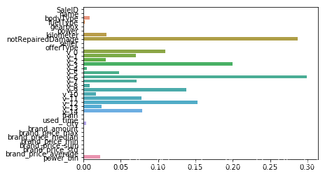
model = Lasso().fit(train_X, train_y_ln)
print('intercept:'+ str(model.intercept_))
sns.barplot(abs(model.coef_), continuous_feature_names)
intercept:7.946156528722565


D:\Software\Anaconda\lib\site-packages\sklearn\linear_model\coordinate_descent.py:492: ConvergenceWarning: Objective did not converge. You might want to increase the number of iterations. Fitting data with very small alpha may cause precision problems.
  ConvergenceWarning)


<matplotlib.axes._subplots.AxesSubplot at 0x210405debe0>
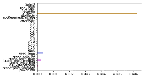
L1正则化有助于生成一个稀疏权值矩阵,进而可以用于特征选择。如上图,我们发现power与userd_time特征非常重要。
3.Ridge方法即L2正则化的情况:
model = Ridge().fit(train_X, train_y_ln)
print('intercept:'+ str(model.intercept_))
sns.barplot(abs(model.coef_), continuous_feature_names)
intercept:2.7820015512913994


<matplotlib.axes._subplots.AxesSubplot at 0x2103fdd99b0>
从上图可以看到有很多参数离0较远,很多为0。
原因在于L2正则化在拟合过程中通常都倾向于让权值尽可能小,最后构造一个所有参数都比较小的模型。因为一般认为参数值小的模型比较简单,能适应不同的数据集,也在一定程度上避免了过拟合现象。
可以设想一下对于一个线性回归方程,若参数很大,那么只要数据偏移一点点,就会对结果造成很大的影响;但如果参数足够小,数据偏移得多一点也不会对结果造成什么影响,专业一点的说法是『抗扰动能力强』
除此之外,决策树通过信息熵或GINI指数选择分裂节点时,优先选择的分裂特征也更加重要,这同样是一种特征选择的方法。XGBoost与LightGBM模型中的model_importance指标正是基于此计算的
4️⃣.2️⃣ 非线性模型
支持向量机,决策树,随机森林,梯度提升树(GBDT),多层感知机(MLP),XGBoost,LightGBM等
from sklearn.linear_model import LinearRegression
from sklearn.svm import SVC
from sklearn.tree import DecisionTreeRegressor
from sklearn.ensemble import RandomForestRegressor
from sklearn.ensemble import GradientBoostingRegressor
from sklearn.neural_network import MLPRegressor
from xgboost.sklearn import XGBRegressor
from lightgbm.sklearn import LGBMRegressor
定义模型集合
models = [LinearRegression(),
          DecisionTreeRegressor(),
          RandomForestRegressor(),
          GradientBoostingRegressor(),
          MLPRegressor(solver='lbfgs', max_iter=100),
          XGBRegressor(n_estimators = 100, objective='reg:squarederror'),
          LGBMRegressor(n_estimators = 100)]
用数据一一对模型进行训练
result = dict()
for model in models:
    model_name = str(model).split('(')[0]
    scores = cross_val_score(model, X=train_X, y=train_y_ln, verbose=0, cv = 5, scoring=make_scorer(mean_absolute_error))
    result[model_name] = scores
    print(model_name + ' is finished')
LinearRegression is finished
DecisionTreeRegressor is finished
RandomForestRegressor is finished
GradientBoostingRegressor is finished
MLPRegressor is finished
XGBRegressor is finished
LGBMRegressor is finished
result = pd.DataFrame(result)
result.index = ['cv' + str(x) for x in range(1, 6)]
result
| LinearRegression | DecisionTreeRegressor | RandomForestRegressor | GradientBoostingRegressor | MLPRegressor | XGBRegressor | LGBMRegressor | |
|---|---|---|---|---|---|---|---|
| cv1 | 0.208238 | 0.224863 | 0.163196 | 0.179385 | 581.596878 | 0.155881 | 0.153942 |
| cv2 | 0.212408 | 0.218795 | 0.164292 | 0.183759 | 182.180288 | 0.158566 | 0.160262 |
| cv3 | 0.215933 | 0.216482 | 0.164849 | 0.185005 | 250.668763 | 0.158520 | 0.159943 |
| cv4 | 0.210742 | 0.220903 | 0.160878 | 0.181660 | 139.101476 | 0.156608 | 0.157528 |
| cv5 | 0.214747 | 0.226087 | 0.164713 | 0.183704 | 108.664261 | 0.173250 | 0.157149 |
可以看到随机森林模型在每一个fold中均取得了更好的效果
np.mean(result['RandomForestRegressor'])
0.16358568277026037
4️⃣.3️⃣ 模型调参
三种常用的调参方法如下:
贪心算法 https://www.jianshu.com/p/ab89df9759c8
网格调参 https://blog.csdn.net/weixin_43172660/article/details/83032029
贝叶斯调参 https://blog.csdn.net/linxid/article/details/81189154
## LGB的参数集合:

objective = ['regression', 'regression_l1', 'mape', 'huber', 'fair']

num_leaves = [3,5,10,15,20,40, 55]
max_depth = [3,5,10,15,20,40, 55]
bagging_fraction = []
feature_fraction = []
drop_rate = []
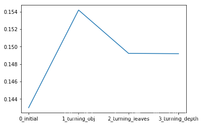
4️⃣.3️⃣.1️⃣ 贪心调参
best_obj = dict()
for obj in objective:
    model = LGBMRegressor(objective=obj)
    score = np.mean(cross_val_score(model, X=train_X, y=train_y_ln, verbose=0, cv = 5, scoring=make_scorer(mean_absolute_error)))
    best_obj[obj] = score

best_leaves = dict()
for leaves in num_leaves:
    model = LGBMRegressor(objective=min(best_obj.items(), key=lambda x:x[1])[0], num_leaves=leaves)
    score = np.mean(cross_val_score(model, X=train_X, y=train_y_ln, verbose=0, cv = 5, scoring=make_scorer(mean_absolute_error)))
    best_leaves[leaves] = score

best_depth = dict()
for depth in max_depth:
    model = LGBMRegressor(objective=min(best_obj.items(), key=lambda x:x[1])[0],
                          num_leaves=min(best_leaves.items(), key=lambda x:x[1])[0],
                          max_depth=depth)
    score = np.mean(cross_val_score(model, X=train_X, y=train_y_ln, verbose=0, cv = 5, scoring=make_scorer(mean_absolute_error)))
    best_depth[depth] = score
sns.lineplot(x=['0_initial','1_turning_obj','2_turning_leaves','3_turning_depth'], y=[0.143 ,min(best_obj.values()), min(best_leaves.values()), min(best_depth.values())])
<matplotlib.axes._subplots.AxesSubplot at 0x21041776128>
4️⃣.3️⃣.2️⃣ Grid Search 网格调参
from sklearn.model_selection import GridSearchCV
parameters = {'objective': objective , 'num_leaves': num_leaves, 'max_depth': max_depth}
model = LGBMRegressor()
clf = GridSearchCV(model, parameters, cv=5)
clf = clf.fit(train_X, train_y)
clf.best_params_
{'max_depth': 10, 'num_leaves': 55, 'objective': 'regression'}
model = LGBMRegressor(objective='regression',
                          num_leaves=55,
                          max_depth=10)
np.mean(cross_val_score(model, X=train_X, y=train_y_ln, verbose=0, cv = 5, scoring=make_scorer(mean_absolute_error)))
0.1526351038235066
4️⃣.3️⃣.3️⃣ 贝叶斯调参
!pip install -i https://pypi.tuna.tsinghua.edu.cn/simple bayesian-optimization
from bayes_opt import BayesianOptimization
Looking in indexes: https://pypi.tuna.tsinghua.edu.cn/simple
Collecting bayesian-optimization
  Downloading https://pypi.tuna.tsinghua.edu.cn/packages/b5/26/9842333adbb8f17bcb3d699400a8b1ccde0af0b6de8d07224e183728acdf/bayesian_optimization-1.1.0-py3-none-any.whl
Requirement already satisfied: scikit-learn>=0.18.0 in d:\software\anaconda\lib\site-packages (from bayesian-optimization) (0.20.3)
Requirement already satisfied: scipy>=0.14.0 in d:\software\anaconda\lib\site-packages (from bayesian-optimization) (1.2.1)
Requirement already satisfied: numpy>=1.9.0 in d:\software\anaconda\lib\site-packages (from bayesian-optimization) (1.16.2)
Installing collected packages: bayesian-optimization
Successfully installed bayesian-optimization-1.1.0
def rf_cv(num_leaves, max_depth, subsample, min_child_samples):
    val = cross_val_score(
        LGBMRegressor(objective = 'regression_l1',
            num_leaves=int(num_leaves),
            max_depth=int(max_depth),
            subsample = subsample,
            min_child_samples = int(min_child_samples)
        ),
        X=train_X, y=train_y_ln, verbose=0, cv = 5, scoring=make_scorer(mean_absolute_error)
    ).mean()
    return 1 - val # 贝叶斯调参目标是求最大值,所以用1减去误差
rf_bo = BayesianOptimization(
    rf_cv,
    {
    'num_leaves': (2, 100),
    'max_depth': (2, 100),
    'subsample': (0.1, 1),
    'min_child_samples' : (2, 100)
    }
)
rf_bo.maximize()
| iter | target | max_depth | min_ch... | num_le... | subsample |
-------------------------------------------------------------------------
| [0m 1 [0m | [0m 0.8493 [0m | [0m 80.61 [0m | [0m 97.58 [0m | [0m 44.92 [0m | [0m 0.881 [0m |
| [95m 2 [0m | [95m 0.8514 [0m | [95m 35.87 [0m | [95m 66.92 [0m | [95m 57.68 [0m | [95m 0.7878 [0m |
| [95m 3 [0m | [95m 0.8522 [0m | [95m 49.75 [0m | [95m 68.95 [0m | [95m 64.99 [0m | [95m 0.1726 [0m |
| [0m 4 [0m | [0m 0.8504 [0m | [0m 35.58 [0m | [0m 10.83 [0m | [0m 53.8 [0m | [0m 0.1306 [0m |
| [0m 5 [0m | [0m 0.7942 [0m | [0m 63.37 [0m | [0m 32.21 [0m | [0m 3.143 [0m | [0m 0.4555 [0m |
| [0m 6 [0m | [0m 0.7997 [0m | [0m 2.437 [0m | [0m 4.362 [0m | [0m 97.26 [0m | [0m 0.9957 [0m |
| [95m 7 [0m | [95m 0.8526 [0m | [95m 47.85 [0m | [95m 69.39 [0m | [95m 68.02 [0m | [95m 0.8833 [0m |
| [95m 8 [0m | [95m 0.8537 [0m | [95m 96.87 [0m | [95m 4.285 [0m | [95m 99.53 [0m | [95m 0.9389 [0m |
| [95m 9 [0m | [95m 0.8546 [0m | [95m 96.06 [0m | [95m 97.85 [0m | [95m 98.82 [0m | [95m 0.8874 [0m |
| [0m 10 [0m | [0m 0.7942 [0m | [0m 8.165 [0m | [0m 99.06 [0m | [0m 3.93 [0m | [0m 0.2049 [0m |
| [0m 11 [0m | [0m 0.7993 [0m | [0m 2.77 [0m | [0m 99.47 [0m | [0m 91.16 [0m | [0m 0.2523 [0m |
| [0m 12 [0m | [0m 0.852 [0m | [0m 99.3 [0m | [0m 43.04 [0m | [0m 62.67 [0m | [0m 0.9897 [0m |
| [0m 13 [0m | [0m 0.8507 [0m | [0m 96.57 [0m | [0m 2.749 [0m | [0m 55.2 [0m | [0m 0.6727 [0m |
| [0m 14 [0m | [0m 0.8168 [0m | [0m 3.076 [0m | [0m 3.269 [0m | [0m 33.78 [0m | [0m 0.5982 [0m |
| [0m 15 [0m | [0m 0.8527 [0m | [0m 71.88 [0m | [0m 7.624 [0m | [0m 76.49 [0m | [0m 0.9536 [0m |
| [0m 16 [0m | [0m 0.8528 [0m | [0m 99.44 [0m | [0m 99.28 [0m | [0m 69.58 [0m | [0m 0.7682 [0m |
| [0m 17 [0m | [0m 0.8543 [0m | [0m 99.93 [0m | [0m 45.95 [0m | [0m 97.54 [0m | [0m 0.5095 [0m |
| [0m 18 [0m | [0m 0.8518 [0m | [0m 60.87 [0m | [0m 99.67 [0m | [0m 61.3 [0m | [0m 0.7369 [0m |
| [0m 19 [0m | [0m 0.8535 [0m | [0m 99.69 [0m | [0m 16.58 [0m | [0m 84.31 [0m | [0m 0.1025 [0m |
| [0m 20 [0m | [0m 0.8507 [0m | [0m 54.68 [0m | [0m 38.11 [0m | [0m 54.65 [0m | [0m 0.9796 [0m |
| [0m 21 [0m | [0m 0.8538 [0m | [0m 99.1 [0m | [0m 81.79 [0m | [0m 84.03 [0m | [0m 0.9823 [0m |
| [0m 22 [0m | [0m 0.8529 [0m | [0m 99.28 [0m | [0m 3.373 [0m | [0m 83.48 [0m | [0m 0.7243 [0m |
| [0m 23 [0m | [0m 0.8512 [0m | [0m 52.67 [0m | [0m 2.614 [0m | [0m 59.65 [0m | [0m 0.5286 [0m |
| [95m 24 [0m | [95m 0.8546 [0m | [95m 75.81 [0m | [95m 61.62 [0m | [95m 99.78 [0m | [95m 0.9956 [0m |
| [0m 25 [0m | [0m 0.853 [0m | [0m 45.9 [0m | [0m 33.68 [0m | [0m 74.59 [0m | [0m 0.73 [0m |
| [0m 26 [0m | [0m 0.8532 [0m | [0m 82.58 [0m | [0m 63.9 [0m | [0m 78.61 [0m | [0m 0.1014 [0m |
| [0m 27 [0m | [0m 0.8544 [0m | [0m 76.15 [0m | [0m 97.58 [0m | [0m 95.07 [0m | [0m 0.9995 [0m |
| [0m 28 [0m | [0m 0.8545 [0m | [0m 95.75 [0m | [0m 74.96 [0m | [0m 99.45 [0m | [0m 0.7263 [0m |
| [0m 29 [0m | [0m 0.8532 [0m | [0m 80.84 [0m | [0m 89.28 [0m | [0m 77.31 [0m | [0m 0.9389 [0m |
| [0m 30 [0m | [0m 0.8545 [0m | [0m 82.92 [0m | [0m 35.46 [0m | [0m 96.66 [0m | [0m 0.969 [0m |
=========================================================================
rf_bo.max
{'target': 0.8545792238909576,
 'params': {'max_depth': 75.80893509302794,
  'min_child_samples': 61.62267920507557,
  'num_leaves': 99.77501502667806,
  'subsample': 0.9955706357612557}}
1 - rf_bo.max['target']
0.14542077610904236
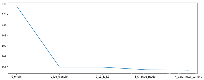
5️⃣ 总结
在本章中,我们完成了建模与调参的工作,并对我们的模型进行了验证。此外,我们还采用了一些基本方法来提高预测的精度,提升如下图所示。
plt.figure(figsize=(13,5))
sns.lineplot(x=['0_origin','1_log_transfer','2_L1_&_L2','3_change_model','4_parameter_turning'], y=[1.36 ,0.19, 0.19, 0.16, 0.15])
<matplotlib.axes._subplots.AxesSubplot at 0x21041688208>
评论区