


1️⃣ 赛题理解✍️
1️⃣.1️⃣ 赛题重述
这是一道来自于天池的新手练习题目,用数据分析、机器学习等手段进行 二手车售卖价格预测 的回归问题。赛题本身的思路清晰明了,即对给定的数据集进行分析探讨,然后设计模型运用数据进行训练,测试模型,最终给出选手的预测结果。
1️⃣.2️⃣ 数据集概述
赛题官方给出了来自Ebay Kleinanzeigen的二手车交易记录,总数据量超过40w,包含31列变量信息,其中15列为匿名变量,即v0至v15。并从中抽取15万条作为训练集,5万条作为测试集A,5万条作为测试集B,同时对name、model、brand和regionCode等信息进行脱敏。具体的数据表如下图:
| Field | Description |
|---|---|
| SaleID | 交易ID,唯一编码 |
| name | 汽车交易名称,已脱敏 |
| regDate | 汽车注册日期,例如20160101,2016年01月01日 |
| model | 车型编码,已脱敏 |
| brand | 汽车品牌,已脱敏 |
| bodyType | 车身类型:豪华轿车:0,微型车:1,厢型车:2,大巴车:3,敞篷车:4,双门汽车:5,商务车:6,搅拌车:7 |
| fuelType | 燃油类型:汽油:0,柴油:1,液化石油气:2,天然气:3,混合动力:4,其他:5,电动:6 |
| gearbox | 变速箱:手动:0,自动:1 |
| power | 发动机功率:范围 [ 0, 600 ] |
| kilometer | 汽车已行驶公里,单位万km |
| notRepairedDamage | 汽车有尚未修复的损坏:是:0,否:1 |
| regionCode | 地区编码,已脱敏 |
| seller | 销售方:个体:0,非个体:1 |
| offerType | 报价类型:提供:0,请求:1 |
| creatDate | 汽车上线时间,即开始售卖时间 |
| price | 二手车交易价格(预测目标) |
| v系列特征 | 匿名特征,包含v0-14在内15个匿名特征 |
思考💭💡
- 指标重要性
- 数据集里面包含的很多维度的数据,对于人来说第一眼看上去就会产生直观的感觉,哪些指标对售价的影响大,哪些指标对售价的影响小,特别是对于一个长期从事二手车交易的人来说,更是如此。例如
kilometer(汽车已行驶公里)肯定是对于成交价格的影响是巨大的。但是如何让我设计的模型认知到这些先验知识是个棘手的问题,但我想这应该时一个很旧的问题,只是我还没有足够的知识去通晓它解决的肌理。确实,对于机器来说,这些数据只是一列列的向量,所以首要解决的就是向量的重要性。
- 数据集里面包含的很多维度的数据,对于人来说第一眼看上去就会产生直观的感觉,哪些指标对售价的影响大,哪些指标对售价的影响小,特别是对于一个长期从事二手车交易的人来说,更是如此。例如
- 简单思维
-
简单地假设(我相信所有人都会想到的easy思路🤪),所有的变量跟预测目标成交价格是simple的线性关系,列一个包含31个自变量的线性函数,用批量梯度下降法拟合出31个自变量系数,然后用正则化解决过拟合问题。
它的假设函数是这样的:
-
它的带有正则化的代价函数是这样的:
1️⃣.3️⃣ 预测结果评价指标⚒️
赛题的预测评估指标为$MAE(Mean Absolute Error)$
可以看出,指标就一个,没有很多维度的评价框架,不那么劝退。🤔
2️⃣ 数据分析EDA📊
- EDA的价值主要在于熟悉数据集,了解数据集,对数据集进行验证来确定所获得数据集可以用于接下来的机器学习或者深度学习使用。
- 当了解了数据集之后我们下一步就是要去了解变量间的相互关系以及变量与预测值之间的存在关系。
- 引导数据科学从业者进行数据处理以及特征工程的步骤,使数据集的结构和特征集让接下来的预测问题更加可靠。
- 完成对于数据的探索性分析,并对于数据进行一些图表或者文字总结并打卡。
当然这一步也要就解决我在 1️⃣.2️⃣ 中提出的第一个思考,能否通过探索性分析,发掘指标之间的关系,从而为模型内联性地定义出各指标的对成交价格的强弱相关性。但是EDA分析涉及的范围太大,可视化的东西很多,但是如果在后续的分析中不进行运用就是多余的工作,所以只需要挑选最重要的几个因素进行分析,具体如下:
- 数据总览,即
describe()统计量以及info()数据类型 - 缺失值以及异常值检测
- 分析待预测的真实值的分布
- 特征之间的相关性分析
2️⃣.1️⃣ 数据总览
2️⃣.1️⃣.1️⃣ 各种计算包的导入
import pandas as pd
import numpy as np
import matplotlib.pyplot as plt
import seaborn as sns # seabon是一个做可视化非常nice的包,它的别名sns是约定俗成的的东西,还有一段很有意思的故事
import missingno as msno # 用来检测缺失值
2️⃣.1️⃣.1️⃣ 数据载入
Train_data = pd.read_csv('used_car_train_20200313.csv', sep=' ')
Test_data = pd.read_csv('used_car_testA_20200313.csv', sep=' ')
2️⃣.1️⃣.2️⃣ 数据的基本形态
- 训练集的长相
Train_data.head()
Train_data.tail()
| SaleID | name | regDate | model | brand | bodyType | fuelType | gearbox | power | kilometer | ... | v_5 | v_6 | v_7 | v_8 | v_9 | v_10 | v_11 | v_12 | v_13 | v_14 | |
|---|---|---|---|---|---|---|---|---|---|---|---|---|---|---|---|---|---|---|---|---|---|
| 149995 | 149995 | 163978 | 20000607 | 121.0 | 10 | 4.0 | 0.0 | 1.0 | 163 | 15.0 | ... | 0.280264 | 0.000310 | 0.048441 | 0.071158 | 0.019174 | 1.988114 | -2.983973 | 0.589167 | -1.304370 | -0.302592 |
| 149996 | 149996 | 184535 | 20091102 | 116.0 | 11 | 0.0 | 0.0 | 0.0 | 125 | 10.0 | ... | 0.253217 | 0.000777 | 0.084079 | 0.099681 | 0.079371 | 1.839166 | -2.774615 | 2.553994 | 0.924196 | -0.272160 |
| 149997 | 149997 | 147587 | 20101003 | 60.0 | 11 | 1.0 | 1.0 | 0.0 | 90 | 6.0 | ... | 0.233353 | 0.000705 | 0.118872 | 0.100118 | 0.097914 | 2.439812 | -1.630677 | 2.290197 | 1.891922 | 0.414931 |
| 149998 | 149998 | 45907 | 20060312 | 34.0 | 10 | 3.0 | 1.0 | 0.0 | 156 | 15.0 | ... | 0.256369 | 0.000252 | 0.081479 | 0.083558 | 0.081498 | 2.075380 | -2.633719 | 1.414937 | 0.431981 | -1.659014 |
| 149999 | 149999 | 177672 | 19990204 | 19.0 | 28 | 6.0 | 0.0 | 1.0 | 193 | 12.5 | ... | 0.284475 | 0.000000 | 0.040072 | 0.062543 | 0.025819 | 1.978453 | -3.179913 | 0.031724 | -1.483350 | -0.342674 |
5 rows × 31 columns
Train_data.shape
(150000, 31)
- 测试集的长相
Test_data.head()
Test_data.tail()
| SaleID | name | regDate | model | brand | bodyType | fuelType | gearbox | power | kilometer | ... | v_5 | v_6 | v_7 | v_8 | v_9 | v_10 | v_11 | v_12 | v_13 | v_14 | |
|---|---|---|---|---|---|---|---|---|---|---|---|---|---|---|---|---|---|---|---|---|---|
| 49995 | 199995 | 20903 | 19960503 | 4.0 | 4 | 4.0 | 0.0 | 0.0 | 116 | 15.0 | ... | 0.284664 | 0.130044 | 0.049833 | 0.028807 | 0.004616 | -5.978511 | 1.303174 | -1.207191 | -1.981240 | -0.357695 |
| 49996 | 199996 | 708 | 19991011 | 0.0 | 0 | 0.0 | 0.0 | 0.0 | 75 | 15.0 | ... | 0.268101 | 0.108095 | 0.066039 | 0.025468 | 0.025971 | -3.913825 | 1.759524 | -2.075658 | -1.154847 | 0.169073 |
| 49997 | 199997 | 6693 | 20040412 | 49.0 | 1 | 0.0 | 1.0 | 1.0 | 224 | 15.0 | ... | 0.269432 | 0.105724 | 0.117652 | 0.057479 | 0.015669 | -4.639065 | 0.654713 | 1.137756 | -1.390531 | 0.254420 |
| 49998 | 199998 | 96900 | 20020008 | 27.0 | 1 | 0.0 | 0.0 | 1.0 | 334 | 15.0 | ... | 0.261152 | 0.000490 | 0.137366 | 0.086216 | 0.051383 | 1.833504 | -2.828687 | 2.465630 | -0.911682 | -2.057353 |
| 49999 | 199999 | 193384 | 20041109 | 166.0 | 6 | 1.0 | NaN | 1.0 | 68 | 9.0 | ... | 0.228730 | 0.000300 | 0.103534 | 0.080625 | 0.124264 | 2.914571 | -1.135270 | 0.547628 | 2.094057 | -1.552150 |
5 rows × 30 columns
Test_data.shape
(50000, 30)
- 可以看出,数据的分散程度很大,有整型,有浮点,有正数,有负数,还有日期,当然可以当成是字符串。另外如果数据都换算成数值的话,数据间差距特别大,有些成千上万,有些几分几厘,这样在预测时就难以避免地会忽视某些值的作用,所以需要对其进行归一化。
shape的运用是也十分重要,对数据的大小要心中有数
- 用
describe()来对数据进行基本统计量的分析,关于describe()的基本参数如下(且其默认只对数值型数据进行分析,如果有字符串,时间序列等的数据,会减少统计的项目):count:一列的元素个数;mean:一列数据的平均值;std:一列数据的均方差;(方差的算术平方根,反映一个数据集的离散程度:越大,数据间的差异越大,数据集中数据的离散程度越高;越小,数据间的大小差异越小,数据集中的数据离散程度越低)min:一列数据中的最小值;max:一列数中的最大值;25%:一列数据中,前 25% 的数据的平均值;50%:一列数据中,前 50% 的数据的平均值;75%:一列数据中,前 75% 的数据的平均值;
- 用
info()来查看数据类型,并主要查看是否有异常数据
Train_data.describe()
| SaleID | name | regDate | model | brand | bodyType | fuelType | gearbox | power | kilometer | ... | v_5 | v_6 | v_7 | v_8 | v_9 | v_10 | v_11 | v_12 | v_13 | v_14 | |
|---|---|---|---|---|---|---|---|---|---|---|---|---|---|---|---|---|---|---|---|---|---|
| count | 150000.000000 | 150000.000000 | 1.500000e+05 | 149999.000000 | 150000.000000 | 145494.000000 | 141320.000000 | 144019.000000 | 150000.000000 | 150000.000000 | ... | 150000.000000 | 150000.000000 | 150000.000000 | 150000.000000 | 150000.000000 | 150000.000000 | 150000.000000 | 150000.000000 | 150000.000000 | 150000.000000 |
| mean | 74999.500000 | 68349.172873 | 2.003417e+07 | 47.129021 | 8.052733 | 1.792369 | 0.375842 | 0.224943 | 119.316547 | 12.597160 | ... | 0.248204 | 0.044923 | 0.124692 | 0.058144 | 0.061996 | -0.001000 | 0.009035 | 0.004813 | 0.000313 | -0.000688 |
| std | 43301.414527 | 61103.875095 | 5.364988e+04 | 49.536040 | 7.864956 | 1.760640 | 0.548677 | 0.417546 | 177.168419 | 3.919576 | ... | 0.045804 | 0.051743 | 0.201410 | 0.029186 | 0.035692 | 3.772386 | 3.286071 | 2.517478 | 1.288988 | 1.038685 |
| min | 0.000000 | 0.000000 | 1.991000e+07 | 0.000000 | 0.000000 | 0.000000 | 0.000000 | 0.000000 | 0.000000 | 0.500000 | ... | 0.000000 | 0.000000 | 0.000000 | 0.000000 | 0.000000 | -9.168192 | -5.558207 | -9.639552 | -4.153899 | -6.546556 |
| 25% | 37499.750000 | 11156.000000 | 1.999091e+07 | 10.000000 | 1.000000 | 0.000000 | 0.000000 | 0.000000 | 75.000000 | 12.500000 | ... | 0.243615 | 0.000038 | 0.062474 | 0.035334 | 0.033930 | -3.722303 | -1.951543 | -1.871846 | -1.057789 | -0.437034 |
| 50% | 74999.500000 | 51638.000000 | 2.003091e+07 | 30.000000 | 6.000000 | 1.000000 | 0.000000 | 0.000000 | 110.000000 | 15.000000 | ... | 0.257798 | 0.000812 | 0.095866 | 0.057014 | 0.058484 | 1.624076 | -0.358053 | -0.130753 | -0.036245 | 0.141246 |
| 75% | 112499.250000 | 118841.250000 | 2.007111e+07 | 66.000000 | 13.000000 | 3.000000 | 1.000000 | 0.000000 | 150.000000 | 15.000000 | ... | 0.265297 | 0.102009 | 0.125243 | 0.079382 | 0.087491 | 2.844357 | 1.255022 | 1.776933 | 0.942813 | 0.680378 |
| max | 149999.000000 | 196812.000000 | 2.015121e+07 | 247.000000 | 39.000000 | 7.000000 | 6.000000 | 1.000000 | 19312.000000 | 15.000000 | ... | 0.291838 | 0.151420 | 1.404936 | 0.160791 | 0.222787 | 12.357011 | 18.819042 | 13.847792 | 11.147669 | 8.658418 |
8 rows × 30 columns
Test_data.describe()
| SaleID | name | regDate | model | brand | bodyType | fuelType | gearbox | power | kilometer | ... | v_5 | v_6 | v_7 | v_8 | v_9 | v_10 | v_11 | v_12 | v_13 | v_14 | |
|---|---|---|---|---|---|---|---|---|---|---|---|---|---|---|---|---|---|---|---|---|---|
| count | 50000.000000 | 50000.000000 | 5.000000e+04 | 50000.000000 | 50000.000000 | 48587.000000 | 47107.000000 | 48090.000000 | 50000.000000 | 50000.000000 | ... | 50000.000000 | 50000.000000 | 50000.000000 | 50000.000000 | 50000.000000 | 50000.000000 | 50000.000000 | 50000.000000 | 50000.000000 | 50000.000000 |
| mean | 174999.500000 | 68542.223280 | 2.003393e+07 | 46.844520 | 8.056240 | 1.782185 | 0.373405 | 0.224350 | 119.883620 | 12.595580 | ... | 0.248669 | 0.045021 | 0.122744 | 0.057997 | 0.062000 | -0.017855 | -0.013742 | -0.013554 | -0.003147 | 0.001516 |
| std | 14433.901067 | 61052.808133 | 5.368870e+04 | 49.469548 | 7.819477 | 1.760736 | 0.546442 | 0.417158 | 185.097387 | 3.908979 | ... | 0.044601 | 0.051766 | 0.195972 | 0.029211 | 0.035653 | 3.747985 | 3.231258 | 2.515962 | 1.286597 | 1.027360 |
| min | 150000.000000 | 0.000000 | 1.991000e+07 | 0.000000 | 0.000000 | 0.000000 | 0.000000 | 0.000000 | 0.000000 | 0.500000 | ... | 0.000000 | 0.000000 | 0.000000 | 0.000000 | 0.000000 | -9.160049 | -5.411964 | -8.916949 | -4.123333 | -6.112667 |
| 25% | 162499.750000 | 11203.500000 | 1.999091e+07 | 10.000000 | 1.000000 | 0.000000 | 0.000000 | 0.000000 | 75.000000 | 12.500000 | ... | 0.243762 | 0.000044 | 0.062644 | 0.035084 | 0.033714 | -3.700121 | -1.971325 | -1.876703 | -1.060428 | -0.437920 |
| 50% | 174999.500000 | 52248.500000 | 2.003091e+07 | 29.000000 | 6.000000 | 1.000000 | 0.000000 | 0.000000 | 109.000000 | 15.000000 | ... | 0.257877 | 0.000815 | 0.095828 | 0.057084 | 0.058764 | 1.613212 | -0.355843 | -0.142779 | -0.035956 | 0.138799 |
| 75% | 187499.250000 | 118856.500000 | 2.007110e+07 | 65.000000 | 13.000000 | 3.000000 | 1.000000 | 0.000000 | 150.000000 | 15.000000 | ... | 0.265328 | 0.102025 | 0.125438 | 0.079077 | 0.087489 | 2.832708 | 1.262914 | 1.764335 | 0.941469 | 0.681163 |
| max | 199999.000000 | 196805.000000 | 2.015121e+07 | 246.000000 | 39.000000 | 7.000000 | 6.000000 | 1.000000 | 20000.000000 | 15.000000 | ... | 0.291618 | 0.153265 | 1.358813 | 0.156355 | 0.214775 | 12.338872 | 18.856218 | 12.950498 | 5.913273 | 2.624622 |
8 rows × 29 columns
Train_data.info()
<class 'pandas.core.frame.DataFrame'>
RangeIndex: 150000 entries, 0 to 149999
Data columns (total 31 columns):
SaleID               150000 non-null int64
name                 150000 non-null int64
regDate              150000 non-null int64
model                149999 non-null float64
brand                150000 non-null int64
bodyType             145494 non-null float64
fuelType             141320 non-null float64
gearbox              144019 non-null float64
power                150000 non-null int64
kilometer            150000 non-null float64
notRepairedDamage    150000 non-null object
regionCode           150000 non-null int64
seller               150000 non-null int64
offerType            150000 non-null int64
creatDate            150000 non-null int64
price                150000 non-null int64
v_0                  150000 non-null float64
v_1                  150000 non-null float64
v_2                  150000 non-null float64
v_3                  150000 non-null float64
v_4                  150000 non-null float64
v_5                  150000 non-null float64
v_6                  150000 non-null float64
v_7                  150000 non-null float64
v_8                  150000 non-null float64
v_9                  150000 non-null float64
v_10                 150000 non-null float64
v_11                 150000 non-null float64
v_12                 150000 non-null float64
v_13                 150000 non-null float64
v_14                 150000 non-null float64
dtypes: float64(20), int64(10), object(1)
memory usage: 35.5+ MB
Test_data.info()
<class 'pandas.core.frame.DataFrame'>
RangeIndex: 50000 entries, 0 to 49999
Data columns (total 30 columns):
SaleID               50000 non-null int64
name                 50000 non-null int64
regDate              50000 non-null int64
model                50000 non-null float64
brand                50000 non-null int64
bodyType             48587 non-null float64
fuelType             47107 non-null float64
gearbox              48090 non-null float64
power                50000 non-null int64
kilometer            50000 non-null float64
notRepairedDamage    50000 non-null object
regionCode           50000 non-null int64
seller               50000 non-null int64
offerType            50000 non-null int64
creatDate            50000 non-null int64
v_0                  50000 non-null float64
v_1                  50000 non-null float64
v_2                  50000 non-null float64
v_3                  50000 non-null float64
v_4                  50000 non-null float64
v_5                  50000 non-null float64
v_6                  50000 non-null float64
v_7                  50000 non-null float64
v_8                  50000 non-null float64
v_9                  50000 non-null float64
v_10                 50000 non-null float64
v_11                 50000 non-null float64
v_12                 50000 non-null float64
v_13                 50000 non-null float64
v_14                 50000 non-null float64
dtypes: float64(20), int64(9), object(1)
memory usage: 11.4+ MB
从上面的统计量与信息来看,没有什么特别之处,就数据类型来说notRepairedDamage的类型是object是个另类,后续要进行特殊处理。
2️⃣.2️⃣ 数据的缺失情况📌
pandas内置了isnull()可以用来判断是否有缺失值,它会对空值和NA进行判断然后返回True或False。
Train_data.isnull().sum()
SaleID                  0
name                    0
regDate                 0
model                   1
brand                   0
bodyType             4506
fuelType             8680
gearbox              5981
power                   0
kilometer               0
notRepairedDamage       0
regionCode              0
seller                  0
offerType               0
creatDate               0
price                   0
v_0                     0
v_1                     0
v_2                     0
v_3                     0
v_4                     0
v_5                     0
v_6                     0
v_7                     0
v_8                     0
v_9                     0
v_10                    0
v_11                    0
v_12                    0
v_13                    0
v_14                    0
dtype: int64
Test_data.isnull().sum()
SaleID                  0
name                    0
regDate                 0
model                   0
brand                   0
bodyType             1413
fuelType             2893
gearbox              1910
power                   0
kilometer               0
notRepairedDamage       0
regionCode              0
seller                  0
offerType               0
creatDate               0
v_0                     0
v_1                     0
v_2                     0
v_3                     0
v_4                     0
v_5                     0
v_6                     0
v_7                     0
v_8                     0
v_9                     0
v_10                    0
v_11                    0
v_12                    0
v_13                    0
v_14                    0
dtype: int64
- 可以看出缺失的数据值主要集中在
bodyType,fuelType,gearbox,这三个特征中。训练集中model缺失了一个值,但是无伤大雅。至于如何填充,亦或是删除这些数据,需要后期在选用模型时再做考虑。 - 同时我们也可以通过
missingno库查看缺省值的其他属性。- 矩阵图
matrix - 柱状图
bar - 热力图
heatmap - 树状图
dendrogram
- 矩阵图
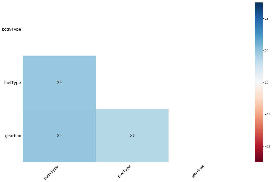
缺省热力图
热力图表示两个特征之间的缺失相关性,即一个变量的存在或不存在如何强烈影响的另一个的存在。如果x和y的热度值是1,则代表当x缺失时,y也百分之百缺失。如果x和y的热度相关性为-1,说明x缺失的值,那么y没有缺失;而x没有缺失时,y为缺失。至于 矩阵图,与柱状图没有查看的必要,我们可以用缺省热力图观察一下情况:
msno.heatmap(Train_data.sample(10000))
<matplotlib.axes._subplots.AxesSubplot at 0x1c62d5c07f0>
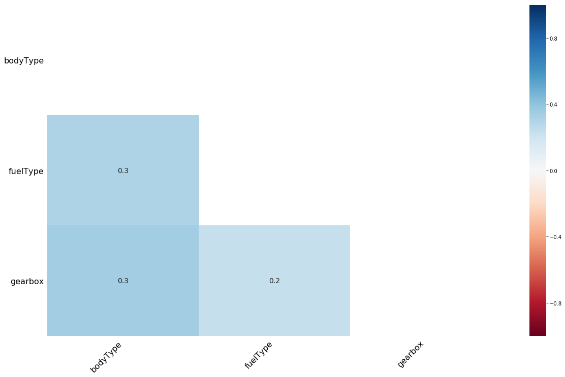
msno.heatmap(Test_data.sample(10000))
<matplotlib.axes._subplots.AxesSubplot at 0x1c62de62d30>
树状图
树形图使用层次聚类算法通过它们的无效性相关性(根据二进制距离测量)将变量彼此相加。在树的每个步骤,基于哪个组合最小化剩余簇的距离来分割变量。变量集越单调,它们的总距离越接近零,并且它们的平均距离(y轴)越接近零。
msno.dendrogram(Train_data.sample(10000))
<matplotlib.axes._subplots.AxesSubplot at 0x1c62de92390>

msno.dendrogram(Test_data.sample(10000))
<matplotlib.axes._subplots.AxesSubplot at 0x1c62d7df400>
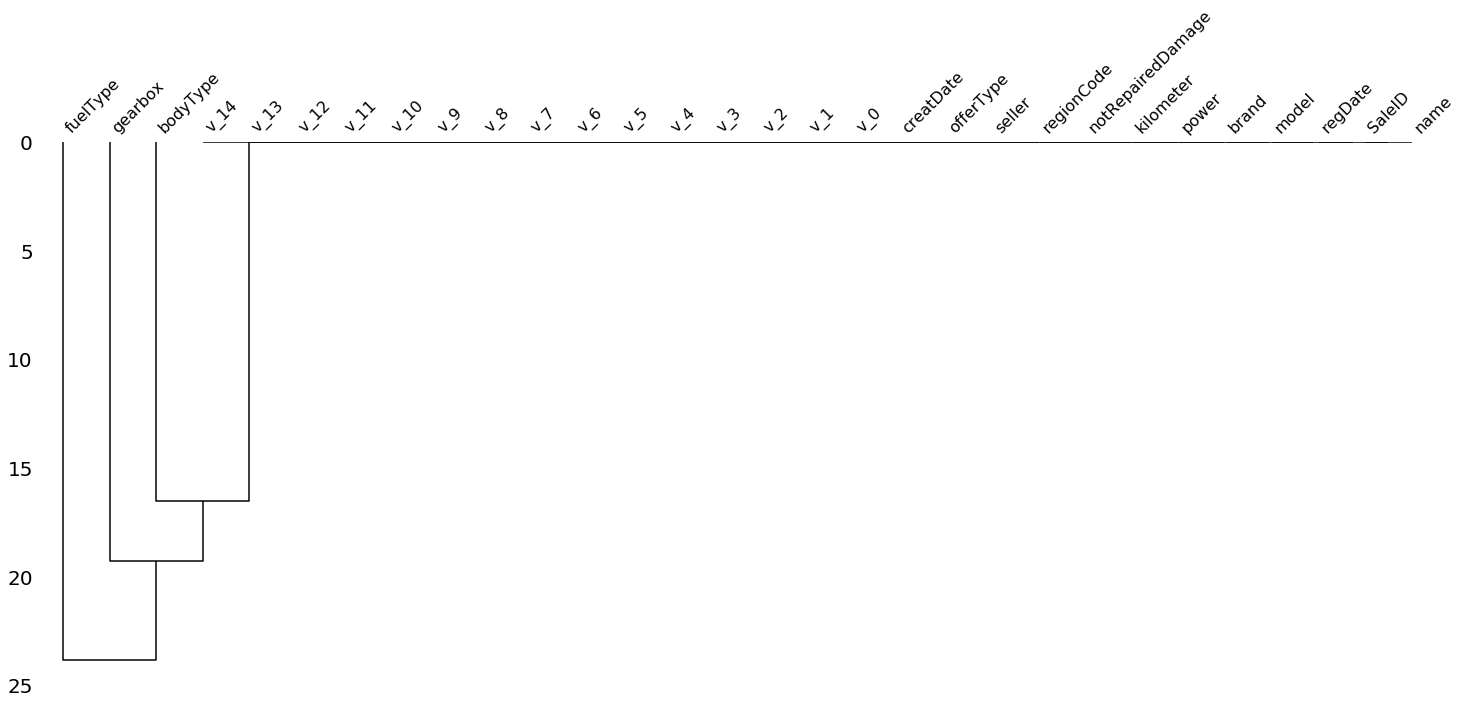
由上面的热力图以及聚类图可以看出,各个缺失值之间的相关性并不明显。
2️⃣.3️⃣ 数据的异常情况☢️
因为之前发现notRepairedDamage的类型是object是个另类,所以看一下它的具体情况。
Train_data['notRepairedDamage'].value_counts()
0.0    111361
-       24324
1.0     14315
Name: notRepairedDamage, dtype: int64
Test_data['notRepairedDamage'].value_counts()
0.0    37249
-       8031
1.0     4720
Name: notRepairedDamage, dtype: int64
发现有'-'的存在,这可以算是NaN的一种,所以可以将其替换为NaN
Train_data['notRepairedDamage'].replace('-', np.nan, inplace=True)
Test_data['notRepairedDamage'].replace('-', np.nan, inplace=True)
2️⃣.4️⃣ 待预测的真实值的分布情况📈
我们先来看看价格预测值的分布情况
Train_data['price']
0         1850
1         3600
2         6222
3         2400
4         5200
          ...
149995    5900
149996    9500
149997    7500
149998    4999
149999    4700
Name: price, Length: 150000, dtype: int64
Train_data['price'].value_counts()
500      2337
1500     2158
1200     1922
1000     1850
2500     1821
         ...
25321       1
8886        1
8801        1
37920       1
8188        1
Name: price, Length: 3763, dtype: int64
嗯哼,平淡无奇,接下来最重要的是要看一下历史成交价格的偏度(Skewness)与峰度(Kurtosis),此外自然界最优美的分布式正态分布,所以也要看一下待预测的价格分布是否满足正态分布。
再解释一下偏度与峰度,一般会拿偏度和峰度来看数据的分布形态,而且一般会跟正态分布做比较,我们把正态分布的偏度和峰度都看做零。如果算到偏度峰度不为0,即表明变量存在左偏右偏,或者是高顶平顶。
- 偏度(Skewness)
是描述数据分布形态的统计量,其描述的是某总体取值分布的对称性,简单来说就是数据的不对称程度。- Skewness = 0 ,分布形态与正态分布偏度相同。
- Skewness > 0 ,正偏差数值较大,为正偏或右偏。长尾巴拖在右边,数据右端有较多的极端值。
- Skewness < 0 ,负偏差数值较大,为负偏或左偏。长尾巴拖在左边,数据左端有较多的极端值。
- 数值的绝对值越大,表明数据分布越不对称,偏斜程度大。
- 计算公式
- 峰度(Kurtosis)
偏度是描述某变量所有取值分布形态陡缓程度的统计量,简单来说就是数据分布顶的尖锐程度。- Kurtosis = 0 与正态分布的陡缓程度相同。
- Kurtosis > 0 比正态分布的高峰更加陡峭——尖顶峰。
- urtosis<0 比正态分布的高峰来得平台——平顶峰。
- 计算公式:
sns.distplot(Train_data['price']);
print("Skewness: %f" % Train_data['price'].skew())
print("Kurtosis: %f" % Train_data['price'].kurt())
Skewness: 3.346487
Kurtosis: 18.995183
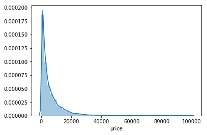
很明显,预测值的数据分布不服从正态分布,偏度与峰度的值都很大,也很符合他们的定义,从图中可以看出,长尾巴拖在右边印证了峰度值很大,峰顶很尖对应了偏度值很大。以我模糊的概率统计知识,这更加像是接近于卡方或者是F分布。所以要对数据本身进行变换。
plt.hist(Train_data['price'], orientation = 'vertical',histtype = 'bar', color ='red')
plt.show()
plt.hist(np.log(Train_data['price']), orientation = 'vertical',histtype = 'bar', color ='red')
plt.show()


由于数据较为集中,这就给预测模型的预测带来比较大的困难,所以可以进行一次log运算改善一下分布,有利于后续的预测。
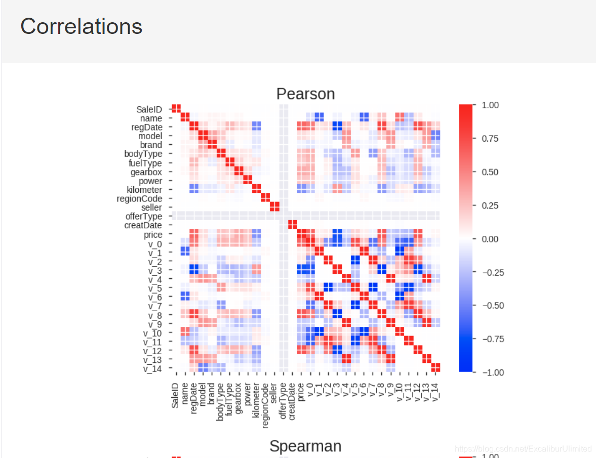
2️⃣.5️⃣ 数据特征相关性的分析🎎
2️⃣.5️⃣.1️⃣ numric特征的相关性分析
这里主要是为了解决我之前提出的疑问,「如何确定每个指标的重要性」,所以研究每个特征之间的相关性就显得尤为重要。在分析之前需要确定哪些特征是numeric型数据,哪些特征是object型数据。自动化的方法是
这样的:
# num_feas = Train_data.select_dtypes(include=[np.number])
# obj_feas = Train_data.select_dtypes(include=[np.object])
但本题的数据集的label已经标好名称了,而且label是有限的,每个种类是可以理解的,所以还是需要人为标注,例如车型bodyType虽然是数值型数据,但其实我们知道它应该是object型数据。所以可以这样:
num_feas = ['power', 'kilometer', 'v_0', 'v_1', 'v_2', 'v_3', 'v_4', 'v_5', 'v_6', 'v_7', 'v_8', 'v_9', 'v_10', 'v_11', 'v_12', 'v_13','v_14' ]

obj_feas = ['name', 'model', 'brand', 'bodyType', 'fuelType', 'gearbox', 'notRepairedDamage', 'regionCode',]
下面我们将price加入num_feas,并用pandas笼统地分析一下特征之间的相关性,并进行可视化。
num_feas.append('price')
price_numeric = Train_data[num_feas]
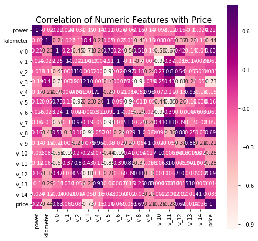
correlation = price_numeric.corr()
print(correlation['price'].sort_values(ascending = False),'\n')
price        1.000000
v_12         0.692823
v_8          0.685798
v_0          0.628397
power        0.219834
v_5          0.164317
v_2          0.085322
v_6          0.068970
v_1          0.060914
v_14         0.035911
v_13        -0.013993
v_7         -0.053024
v_4         -0.147085
v_9         -0.206205
v_10        -0.246175
v_11        -0.275320
kilometer   -0.440519
v_3         -0.730946
Name: price, dtype: float64
f , ax = plt.subplots(figsize = (8, 8))
plt.title('Correlation of Numeric Features with Price', y = 1, size = 16)
sns.heatmap(correlation, square = True, annot=True, cmap='RdPu', vmax = 0.8) # 参数annot为True时,为每个单元格写入数据值。如果数组具有与数据相同的形状,则使用它来注释热力图而不是原始数据。
<matplotlib.axes._subplots.AxesSubplot at 0x1c63234b400>
作为一个色彩控,cmap的可选参数有Accent, Accent_r, Blues, Blues_r, BrBG, BrBG_r, BuGn, BuGn_r, BuPu, BuPu_r, CMRmap, CMRmap_r, Dark2, Dark2_r, GnBu, GnBu_r, Greens, Greens_r, Greys, Greys_r, OrRd, OrRd_r, Oranges, Oranges_r, PRGn, PRGn_r, Paired, Paired_r, Pastel1, Pastel1_r, Pastel2, Pastel2_r, PiYG, PiYG_r, PuBu, PuBuGn, PuBuGn_r, PuBu_r, PuOr, PuOr_r, PuRd, PuRd_r, Purples, Purples_r, RdBu, RdBu_r, RdGy, RdGy_r, RdPu, RdPu_r, RdYlBu, RdYlBu_r, RdYlGn, RdYlGn_r, Reds, Reds_r, Set1, Set1_r, Set2, Set2_r, Set3, Set3_r, Spectral, Spectral_r, Wistia, Wistia_r, YlGn, YlGnBu, YlGnBu_r, YlGn_r, YlOrBr, YlOrBr_r, YlOrRd, YlOrRd_r...其中末尾加r是颜色取反。
关于seaborn的heatmap可以看这里seaborn.heatmap的初步学习
言归正传,从热度图中可以看出跟price相关性高的几个特征主要包括:kilometer,v3。与我们的现实经验还是比较吻合的,那个v3可能是发动机等汽车重要部件相关的某个参数。
- 峰度与偏度
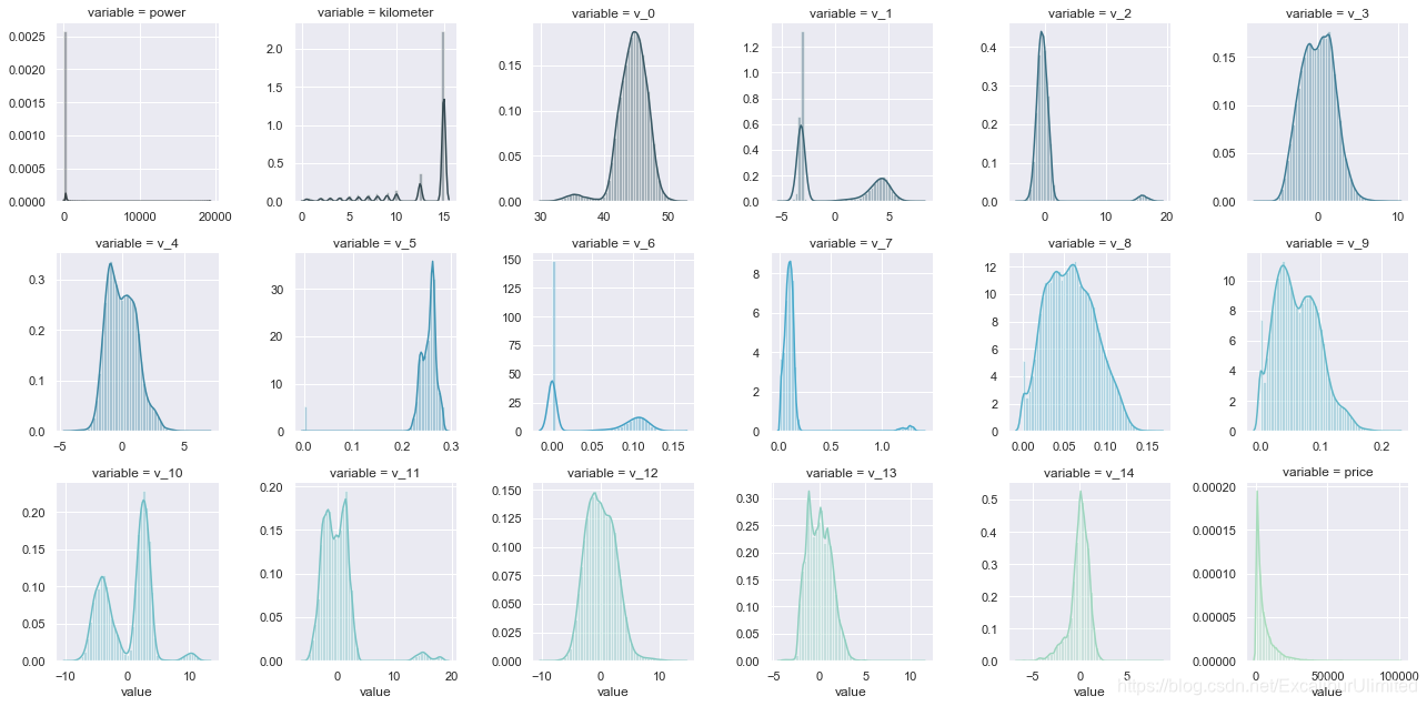
查看各个特征的偏度与峰度,以及数据的分布状况
del price_numeric['price']
#  输出数据的峰度与偏度,这里pandas可以直接调用
for col in num_feas:
    print('{:15}'.format(col),
          'Skewness: {:05.2f}'.format(Train_data[col].skew()) ,
          '   ' ,
          'Kurtosis: {:06.2f}'.format(Train_data[col].kurt())
         )

f = pd.melt(Train_data, value_vars = num_feas) # 利用pandas的melt函数将测试集中的num_feas所对应的数据取出来
# FacetGrid是sns库中用来画网格图的函数,其中col_wrap用来控制一行显示图的个数,sharex或者sharey是否共享x,y轴,意味着每个子图是否有自己的横纵坐标。
g = sns.FacetGrid(f, col = "variable",  col_wrap = 6, sharex = False, sharey = False, hue = 'variable', palette = "GnBu_d") # palette的可选参数与上文的cmap类似
g = g.map(sns.distplot, "value")
power           Skewness: 65.86     Kurtosis: 5733.45
kilometer       Skewness: -1.53     Kurtosis: 001.14
v_0             Skewness: -1.32     Kurtosis: 003.99
v_1             Skewness: 00.36     Kurtosis: -01.75
v_2             Skewness: 04.84     Kurtosis: 023.86
v_3             Skewness: 00.11     Kurtosis: -00.42
v_4             Skewness: 00.37     Kurtosis: -00.20
v_5             Skewness: -4.74     Kurtosis: 022.93
v_6             Skewness: 00.37     Kurtosis: -01.74
v_7             Skewness: 05.13     Kurtosis: 025.85
v_8             Skewness: 00.20     Kurtosis: -00.64
v_9             Skewness: 00.42     Kurtosis: -00.32
v_10            Skewness: 00.03     Kurtosis: -00.58
v_11            Skewness: 03.03     Kurtosis: 012.57
v_12            Skewness: 00.37     Kurtosis: 000.27
v_13            Skewness: 00.27     Kurtosis: -00.44
v_14            Skewness: -1.19     Kurtosis: 002.39
price           Skewness: 03.35     Kurtosis: 019.00
各个数值特征之间的相关性
sns.set()
columns = num_feas
sns.pairplot(Train_data[columns], size = 2 , kind = 'scatter', diag_kind ='kde', palette = "PuBu")
plt.show()
D:\Software\Anaconda\lib\site-packages\seaborn\axisgrid.py:2065: UserWarning: The `size` parameter has been renamed to `height`; pleaes update your code.
  warnings.warn(msg, UserWarning)

可以看出成闭团状的相关图还是很多的,说明相应特征的相关度比较大。
price与其他变量相关性可视化
这里用匿名变量v0~v13进行分析,使用seaborn的regplot函数进行相关度回归分析。
Y_train = Train_data['price']
fig, ((ax1, ax2), (ax3, ax4), (ax5, ax6), (ax7, ax8), (ax9, ax10),(ax11, ax12),(ax13,ax14)) = plt.subplots(nrows = 7, ncols=2, figsize=(24, 20))
ax = [ax1, ax2, ax3, ax4, ax5, ax6, ax7, ax8, ax9, ax10, ax11, ax12, ax13, ax14]
for num in range(0,14):
    sns.regplot(x = 'v_' + str(num), y = 'price', data = pd.concat([Y_train, Train_data['v_' + str(num)]],axis = 1), scatter = True, fit_reg = True, ax = ax[num])
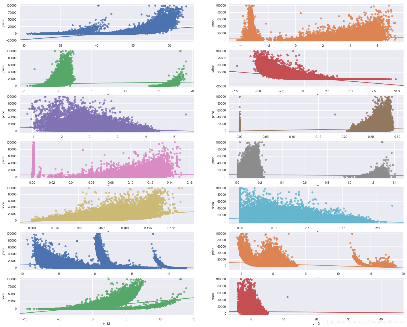
可以看出大部分匿名变量的分布还是比较集中的,当然线性回归的性能确实太弱了。
至于类别特征的回归分析,本身可以参考的意义不大,就暂时省略了。
2️⃣.5️⃣.2️⃣ pandas_profiling生成数据报告📕
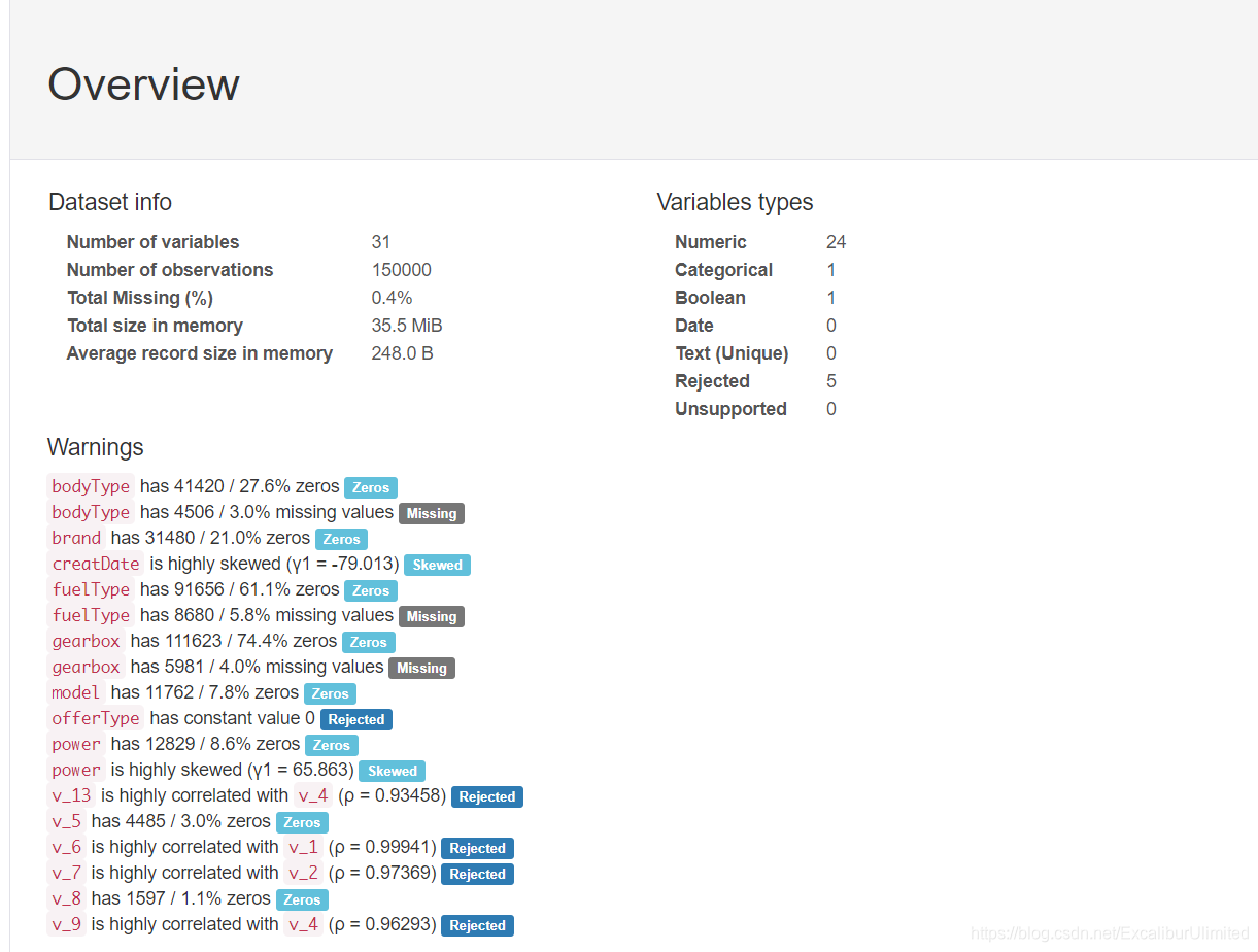
用pandas_profiling生成一个较为全面的可视化和数据报告(较为简单、方便)最终打开html文件即可
import pandas_profiling
file = pandas_profiling.ProfileReport(Train_data)
pfr.to_file("pandas_analysis.html")
长这个样子:
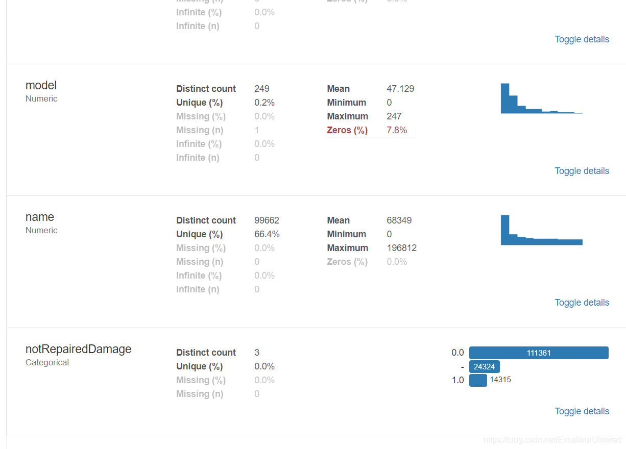
具体文件在这里我的天池
3️⃣ 结语✏️
至此赛题的赛题理解以及数据分析工作告一段落,总结一下:
- 运用
describe()和info()进行数据基本统计量的描述 - 运用
missingno库和pandas.isnull()来对异常值和缺失值进行可视化察觉以及处理 - 熟悉偏度(Skewness)与峰度(Kurtosis)的概念,可以用
skeu()和kurt()计算其值 - 在确定预测值的范围与分布后,可以做一些取对数或者开根号的方式缓解数据集中的问题
- 相关性分析时
- 用
corr()计算各特征的相关系数 - 用
seaborn的heatmap画出相关系数的热力图 - 用
seaborn的FacetGrid和pairplot可以分别画出各特征内部之间以及预测值与其他特征之间的数据分布图 - 也可以用
seaborn的regplot来对预测值与各特征的关系进行回归分析
- 用
开始下一步特征工程。
评论区